Predicting horror movie ratings with LASSO regression

Setup

First, we’ll load the tidyverse and a few other packages:

• lubridate to work with dates
• tidytext to work with text and create sparse matrixes
• glmnet to run LASSO regression
• scales to turn numbers into pretty numbers (e.g., 3000 to 3,000)
• glue to incorporate dynamic data into graph title and annotations

library(tidyverse)
library(lubridate)
library(tidytext)
library(glmnet)
library(scales)
library(glue)

theme_set(theme_light())

horror_movies_raw <- readr::read_csv("https://raw.githubusercontent.com/rfordatascience/tidytuesday/master/data/2019/2019-10-22/horror_movies.csv")

Data inspection

Let’s see what we have.

horror_movies_raw %>%
  glimpse()

## Rows: 3,328
## Columns: 12
## $ title             <chr> "Gut (2012)", "The Haunting of Mia Moss (2017)", ...
## $ genres            <chr> "Drama| Horror| Thriller", "Horror", "Horror", "C...
## $ release_date      <chr> "26-Oct-12", "13-Jan-17", "21-Oct-17", "23-Apr-13...
## $ release_country   <chr> "USA", "USA", "Canada", "USA", "USA", "UK", "USA"...
## $ movie_rating      <chr> NA, NA, NA, "NOT RATED", NA, NA, "NOT RATED", NA,...
## $ review_rating     <dbl> 3.9, NA, NA, 3.7, 5.8, NA, 5.1, 6.5, 4.6, 5.4, 5....
## $ movie_run_time    <chr> "91 min", NA, NA, "82 min", "80 min", "93 min", "...
## $ plot              <chr> "Directed by Elias. With Jason Vail, Nicholas Wil...
## $ cast              <chr> "Jason Vail|Nicholas Wilder|Sarah Schoofs|Kirstia...
## $ language          <chr> "English", "English", "English", "English", "Ital...
## $ filming_locations <chr> "New York, USA", NA, "Sudbury, Ontario, Canada", ...
## $ budget            <chr> NA, "$30,000", NA, NA, NA, "$3,400,000", NA, NA, ...

The unit of observation is a movie, and each movie has three data types associated with it:

1. Continuous or ordered discrete: all the fields with numbers, like movie_run_time, movie_rating, and release_date.
2. Categorical: almost all the rest of the fields, like genres and language. filming_locations is a bit special because it’s hierarchical (e.g., “Sudbury, Ontario, Canada” has city, province, and country in it).
3. Free text: plot is contains cast information and a plot synopsis. We might do something interesting with this field later.
    

Let’s look at one of the plot descriptions by using the sample_n function to randomly select one row, then select just the title and plot. I quickly scanned the list and picked one out with a ridiculous title: Sorority Slaughterhouse.

horror_movies_raw %>%
  filter(str_detect(title, "Sorority Slaughterhouse")) %>%
  select(title, plot) %>%
  knitr::kable(format = "html")

Wow. My idea of a horror movie is The Sixth Sense, which seems extremely tame compared to Sorority Slaughterhouse.
 

Let’s move on and and check fields for missing values. Our glimpse above showed a few fields that looked like they had a lot of them.

horror_movies_raw %>%
  summarise_all(~ mean(is.na(.))) %>%
  gather("field", "pct_missing") %>%
  arrange(-pct_missing)

## # A tibble: 12 x 2
##    field             pct_missing
##    <chr>                   <dbl>
##  1 budget               0.629   
##  2 movie_rating         0.564   
##  3 filming_locations    0.370   
##  4 movie_run_time       0.163   
##  5 review_rating        0.0757  
##  6 language             0.0213  
##  7 cast                 0.00421 
##  8 genres               0.000300
##  9 plot                 0.000300
## 10 title                0       
## 11 release_date         0       
## 12 release_country      0

Three fields – budget, movie_rating, and filming_locations – are missing for between a third and two-thirds of movies. Rather than worry too much about these, I’m going to drop them. Besides, dealing with the different currencies in budget would be a major pain. Imagine finding the conversion rates for all those different date and currencies to get them all to the same currency. Hard pass.
 

Research question

It’s practically data science law that when you have a movie dataset that includes ratings, you have to build a model to predict ratings. There’s a fair bit of data here, with a lot more variety in language and release country than you see in many movie datasets.

review_rating, the field we’ll be trying to predict, has some missing values – about 7%. If we were analyzing this dataset in details we’d want to dig into these missing values to see if there is a systemic reason they are missing. But since this is just a fun, quick exploration, we’ll ignore them.
 

Data cleaning

You may have noticed that this data is a bit messy, with numbers coded as characters (movie_run_time), dates as characters (release_date), and fields with multiple values in one observation (genres). That just means it will make for a fun cleaning exercise. We’re going to:

1. Filter out the missing review_rating observations.
2. Get rid of duplicate observations – there are 16 of them.
3. Add an id field. I almost always do this if one doesn’t already exist because it ensures we have a unique key. It’s helpful for this dataset because there are some different movies that have the same title. Adding an id helps prevent issues if we decided to aggregate the data.
4. Separate movie title and release year from the title field.
5. Convert movie_run_time to a proper number.
6. Scrub the first line of plot (“Directed by…”) to get a “clean” plot synopsis.
7. Ditch movie_rating, filming_location, and budget. They have too much missing data or are too messy to be immediately useful to us.
8. Ditch release_date, too. The data looks fine – but having just the release year will be enough for us.

horror_movies <- horror_movies_raw %>%
  filter(!is.na(review_rating)) %>%
  distinct(title, plot, .keep_all = TRUE) %>%
  mutate(id = row_number(),
         # Pull out any series of four digits - i.e., release year
         release_year = parse_number(str_extract(title, "\\([0-9]{4}\\)")),
         # Remove those digits we just pulled out
         title = str_remove(title, " \\([0-9]{4}\\)"),
         release_date = dmy(release_date),
         movie_run_time = parse_number(movie_run_time),
         # Pull out text between "Directed by" and ". With"
         director = str_extract(plot, "(?<=Directed by )(.*?)(?=\\. With)"),
         # Remove "Directed by" and "With [cast]" sentences
         plot = str_squish(str_remove(plot, "Directed by.*?\\. With.*?\\."))) %>%
  select(-movie_rating, -filming_locations, -budget, -release_date)

Great! We’re almost ready to build a model. We’re going to use a movie’s features, like director, genre, cast, and language, to predict its rating. To do that with LASSO regression, we need to build a matrix where each row is a movie and each column is a feature. The values in the matrix will answer the question, “Does [this movie] have [this feature]?” A value of 1 means “Yes” and 0 means “No”.

A matrix is two-dimensional, though (1 row + 1 column = 2 dimensions), so we need get our dataset into two dimensions before we convert it to a matrix. We want to end up with two fields – id and feature – that correspond to the rows and columns of the matrix. id is already its own field, but feature is spread across several different fields, so we need to collect them, which we’ll do in three steps:

1. Use the pivot_longer to turn data from a wide to a long format. This will get all features condensed to two fields: feature, which will be the former field name (e.g., country), and value, which will be the value for that observation (e.g., USA).
2. Use the separate_rows functions to further separate some fields. For example, cast has multiple cast members separated by a pipe charcter |.
3. Combine the feature and value fields created in Step 1 so that we have a single field (e.g., “Country: USA”) to turn into a matrix.

by_feature <- horror_movies %>%
  # Select only fields we need, using transmute to rename and re-order
  transmute(id,
            title,
            # Convert to character to avoid uniting different data classes
            year = as.character(release_year),
            director,
            country = release_country,
            cast,
            language,
            genre = genres,
            rating = review_rating) %>%
  # 1. Convert to long format
  pivot_longer(year:genre, names_to = "feature") %>%
  # 2. Further separate delimited values
  separate_rows(value, sep = "\\|") %>%
  # Capitalize some words and get rid of extra whitespace
  mutate(feature = str_to_title(feature),
         value = str_squish(value)) %>%
  # 3. Combine feature and value into one field
  unite(feature, feature, value, sep = ": ")

Modelling

We’re ready to build our LASSO model! Let’s see what our pre-matrix dataset looks like for Sorority Slaughterhouse.

by_feature %>%
  filter(title == "Sorority Slaughterhouse")

## # A tibble: 13 x 4
##       id title                   rating feature                     
##    <int> <chr>                    <dbl> <chr>                       
##  1  1722 Sorority Slaughterhouse    3.3 Year: 2016                  
##  2  1722 Sorority Slaughterhouse    3.3 Director: David DeCoteau    
##  3  1722 Sorority Slaughterhouse    3.3 Country: USA                
##  4  1722 Sorority Slaughterhouse    3.3 Cast: Eric Roberts          
##  5  1722 Sorority Slaughterhouse    3.3 Cast: Jessica Morris        
##  6  1722 Sorority Slaughterhouse    3.3 Cast: Jean Louise O'Sullivan
##  7  1722 Sorority Slaughterhouse    3.3 Cast: Anthony Caravella     
##  8  1722 Sorority Slaughterhouse    3.3 Cast: Alexia Quinn          
##  9  1722 Sorority Slaughterhouse    3.3 Cast: Brianna Joy Chomer    
## 10  1722 Sorority Slaughterhouse    3.3 Cast: Kelli Seymour         
## 11  1722 Sorority Slaughterhouse    3.3 Cast: Vince Hill-Bedford    
## 12  1722 Sorority Slaughterhouse    3.3 Language: English           
## 13  1722 Sorority Slaughterhouse    3.3 Genre: Horror

Everything looks neat and tidy. We can see each feature that Sorority Slaughterhouse has. All of these will get a value of 1 once we convert this to a matrix. So let’s go ahead and create our matrix.

feature_matrix <- by_feature %>%
  # We don't technically need title, just id and feature
  select(id, feature) %>%
  cast_sparse(id, feature)

# Take a look at part of our matrix
feature_matrix[200:210, 19:22]

## 11 x 4 sparse Matrix of class "dgCMatrix"
##     Language: English Genre: Drama Genre: Horror Genre: Thriller
## 200                 1            .             1               .
## 201                 1            .             1               .
## 202                 1            1             1               .
## 203                 1            .             1               .
## 204                 1            1             1               .
## 205                 1            .             1               1
## 206                 1            .             1               .
## 207                 1            .             1               .
## 208                 1            .             1               1
## 209                 1            .             1               1
## 210                 .            .             1               .

Looking at 10 sample rows of the matrix, we see how it is structured:

• All but one movie is in English
• Two movies are Dramas
• All movies are Horror (duh)
• Three movies are Thrillers
   

One last step before we build the model. We have all our predictors in this matrix (the features), but we still need the rating – the thing we’re trying to predict! I don’t know of an elegant way to do this, so we’ll have to rely on some base R code instead of beautiful tidyverse functions.

# Get vector of movie id, which are row names of our matrix
ids <- as.integer(rownames(feature_matrix))

# Look up those ids in horror_movies to get a vector of actual ratings
ratings <- horror_movies$review_rating[ids]

We can finally build our LASSO model, which we’ll do using the glmnet package. We’ll use the cv.glmnet function, which builds a cross-validated LASSO model. It needs two arguments, though we’ll be using three:

• x: matrix of predictors, which in our case is feature_matrix.
• y: Vector of responses (the thing you’re trying to predict), which in our case is ratings.
• nfolds (optional): Number of folds to use in cross-validation. We’ll use 100 since our dataset is not that big.

After building our model, we’re going to select version that has the lowest mean-squared error and get it into a nice format using the broom package’s tidy function.

set.seed(24601)

cv_lasso_model <- cv.glmnet(feature_matrix, # Predictors (features)
                            ratings, # Response variable (ratings)
                            nfolds = 100) # Folds for cross-validation

cv_lasso_model_tidy <- cv_lasso_model$glmnet.fit %>%
  tidy() %>%
  filter(lambda == cv_lasso_model$lambda.min)

cv_lasso_model_tidy

## # A tibble: 1,031 x 5
##    term                  step estimate lambda dev.ratio
##    <chr>                <dbl>    <dbl>  <dbl>     <dbl>
##  1 (Intercept)             41   5.23   0.0382     0.412
##  2 Year: 2012              41  -0.117  0.0382     0.412
##  3 Language: English       41  -0.492  0.0382     0.412
##  4 Genre: Drama            41   0.332  0.0382     0.412
##  5 Cast: Veronica Ricci    41  -0.374  0.0382     0.412
##  6 Genre: Comedy           41   0.208  0.0382     0.412
##  7 Genre: Crime            41   0.234  0.0382     0.412
##  8 Cast: Nao Ohmori        41   0.0187 0.0382     0.412
##  9 Language: Japanese      41   0.0602 0.0382     0.412
## 10 Genre: Mystery          41   0.204  0.0382     0.412
## # ... with 1,021 more rows

Our model has a whopping 1,030 predictors! (Intercept) shows the “starting” rating before we take features into account. Then we add whatever value is in the estimate field for each feature that a movie has. We end up with that movie’s a predicted rating For example, if a movie is a Drama it will get 0.332 added to its predicted rating, while a movie with Veronica Ricci in its cast will get 0.374 subtracted from its predicted rating.

If we join the cv_lasso_model_tidy dataset to our by_feature dataset, we can get predicted values for each movie. Let’s see how Sorority Slaugherhouse does.

sorority <- by_feature %>%
  filter(title == "Sorority Slaughterhouse") %>%
  left_join(cv_lasso_model_tidy, by = c("feature" = "term")) %>%
  replace_na(list(estimate = 0))

sorority %>%
  mutate(direction = ifelse(estimate > 0, "Positive", "Negative"),
         feature = fct_reorder(feature, estimate)) %>%
  ggplot(aes(feature, estimate, fill = direction)) +
  geom_col() +
  geom_hline(aes(yintercept = 0), col = "black") +
  coord_flip() +
  scale_fill_manual(values = c("#b2182b", "#053061")) +
  theme(legend.position = "none",
        panel.grid.minor = element_blank()) +
  labs(title = "Predicting Sorority Slaughterhouse's rating",
       subtitle = "Based on a LASSO regression model",
       x = "",
       y = "Effect on predicted rating")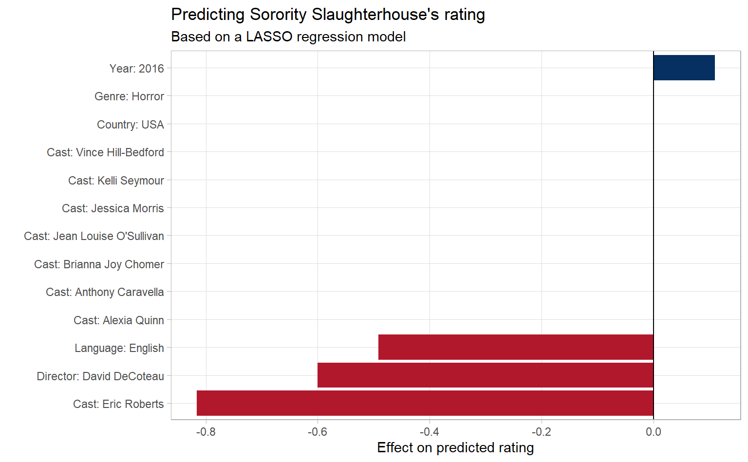

Amazing. Most features didn’t have any effect on the predicted rating, which means they didn’t make it into the LASSO model. But a few features had a big negative impact on the predicted rating. I guess movies in English, directed by David DeCoteau, with Eric Roberts in the cast haven’t done so great in the past. How does our prediction stack up?

base_score <- cv_lasso_model_tidy %>%
  filter(term == "(Intercept)") %>%
  pull(estimate)

by_feature %>%
  filter(title == "Sorority Slaughterhouse") %>%
  inner_join(cv_lasso_model_tidy, by = c("feature" = "term")) %>%
  group_by(title, rating) %>%
  summarise(predicted_rating = base_score + sum(estimate)) %>%
  ungroup()

## `summarise()` regrouping output by 'title' (override with `.groups` argument)

## # A tibble: 1 x 3
##   title                   rating predicted_rating
##   <chr>                    <dbl>            <dbl>
## 1 Sorority Slaughterhouse    3.3             3.43

Pretty good! We successfully identified a bad movie.
 

Visualization

Let’s look at our model in general. I want to know which of the 1,030 features in our model have the biggest positive and negative impact on predicted score.

(Note: We’re going to use the glue package, to dynamically give the number of movies and base score in our chosen LASSO model. This isn’t strictly necessary – we could look it up and hardcode it into our labels – but it’s a cool trick and makes for a slightly more reproduceable analysis. For a quick look at what glue does, check out Sharla Gelfand’s example here.)

cv_lasso_model_tidy %>%
  filter(term != "(Intercept)") %>%
  group_by(direction = ifelse(estimate > 0, "Positive", "Negative")) %>%
  top_n(12, abs(estimate)) %>%
  ungroup() %>%
  mutate(term = fct_reorder(term, estimate)) %>%
  ggplot(aes(term, estimate, fill = direction)) +
  geom_col() +
  coord_flip() +
  scale_fill_manual(values = c("#b2182b", "#053061")) +
  theme(legend.position = "none") +
  labs(title = "How do cast, language, and release country affect rating?",
       subtitle = glue("Lasso fit model of ratings for {comma(length(ids))} horror movies"),
       x = "",
       y = glue('Effect on predicted rating (starting with a base rating of {cv_lasso_model_tidy %>% filter(term == "(Intercept)") %>% pull(estimate) %>% round(1)})'))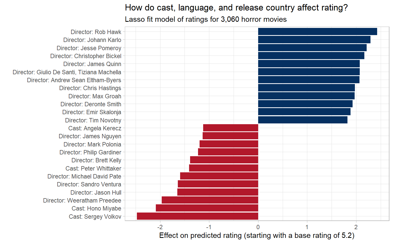

Based on what our model is telling us, director has the biggest impact on predicted rating. Almost every top feature, both positive and negative, is who directed it. I guess there’s something to be said for a director with (or without) a vision.

If Rob Hawk is the “best” director (according to our model) what movie should I watch this Halloween?

by_feature %>%
  filter(feature == "Director: Rob Hawk")

## # A tibble: 1 x 4
##      id title                rating feature           
##   <int> <chr>                 <dbl> <chr>             
## 1   671 Take 2: The Audition    9.3 Director: Rob Hawk

Take 2: The Audition it is!
 

Conclusion

If you liked this, check out the #TidyTuesday hashtag on Twitter. People make truly wonderful contributions every week. Even better would be to participate in TidyTuesday. The R community is tremendously positive and supportive.