Mapping San Francisco's trees

Jan 29, 2020

TidyTuesday / geographic maps / small multiples / tutorial

In this post, I create some basic geographical maps using the San Francisco Trees dataset from TidyTuesday, a project that shares a new dataset each wee to give R users a way to apply and practice their skills.

Getting started with geographical mapping in R can be daunting because there is a lot of terminology to describe a lot of methods that are specific to mapping. There is a whole discipline – Geographic Information Systems – dedicated to this stuff, so it’s no surprise that it can get complicated fast.

We’ll keep things simple. We’re going to map two things: tree locations and roads.

Setup

We’ll start by loading the tidyverse and the sf package, which we’ll use to work with shapefiles, a common format for geospatial data. If the term shapefile is new to you, don’t worry – we’ll cover what it is and how to use it.

library(tidyverse)
library(sf)

theme_set(theme_light())

sf_trees_raw <- readr::read_csv('https://raw.githubusercontent.com/rfordatascience/tidytuesday/master/data/2020/2020-01-28/sf_trees.csv')

Data inspection

Let’s take a look!

sf_trees_raw %>%
  glimpse()

## Rows: 192,987
## Columns: 12
## $ tree_id      <dbl> 53719, 30313, 30312, 30314, 30315, 30316, 48435, 30319...
## $ legal_status <chr> "Permitted Site", "Permitted Site", "Permitted Site", ...
## $ species      <chr> "Tree(s) ::", "Tree(s) ::", "Tree(s) ::", "Pittosporum...
## $ address      <chr> "2963 Webster St", "501 Arkansas St", "501 Arkansas St...
## $ site_order   <dbl> 1, 3, 2, 1, 5, 6, 4, 2, 1, 3, 1, 3, 1, 2, 4, 1, 1, 1, ...
## $ site_info    <chr> "Sidewalk: Curb side : Cutout", "Sidewalk: Curb side :...
## $ caretaker    <chr> "Private", "Private", "Private", "Private", "Private",...
## $ date         <date> 1955-09-19, 1955-10-20, 1955-10-20, 1955-10-20, 1955-...
## $ dbh          <dbl> NA, NA, NA, 16, NA, NA, NA, NA, NA, NA, 2, NA, NA, NA,...
## $ plot_size    <chr> NA, NA, NA, NA, NA, NA, NA, NA, NA, NA, NA, NA, NA, NA...
## $ latitude     <dbl> 37.79787, 37.75984, 37.75984, 37.75977, 37.79265, 37.7...
## $ longitude    <dbl> -122.4341, -122.3981, -122.3981, -122.3981, -122.4124,...

Our unit of observation is a tree – one row corresponds to one tree – and there are three types of data:

Tree data, like what species it is, when it was planted, and who is responsible for maintaing it.
Site data, like a physical description (e.g., sidewalk) and the size of the plot.
Location data, like address and, importantly for us, longitude and latitude coordinates.

We have longitude and latitude, which essentially correspond to the x-axis and y-axis, so let’s start with a scatter plot of tree locations. We have almost 200,000 observations, so we’ll use a period . as a custom shape to avoid overplotting.

sf_trees_raw %>%
  ggplot(aes(longitude, latitude)) +
  geom_point(shape = ".")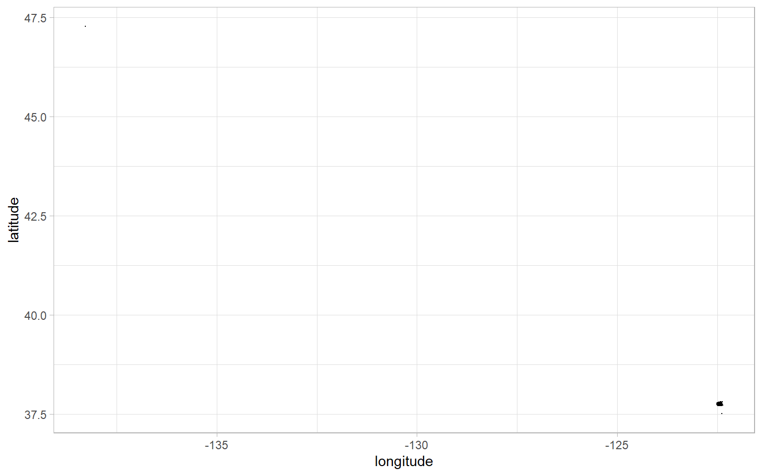

That’s not very informative. There is a tiny cluster of dots in the lower-right, our latitude goes as high as around 47, and our longitude goes as low as around -135. There is data in these ranges, otherwise the graph wouldn’t extend the axes this far. I suspect that we have some miscoded outliers because, as a Canadian, I know for a fact that San Francisco is nowhere near the 49th parallel.

Let’s create boxplots of latitude and longitude. I want to see both graphs side-by-side, so we’ll use the gather() function to get them from having their own column to their own row. Then, we can use facet_wrap() to give each one its own graph.

sf_trees_raw %>%
  select(tree_id, latitude, longitude) %>%
  gather(measure, value, -tree_id) %>%
  # Set x = 1 because we need to give ggplot some value for x
  ggplot(aes(1, value)) +
  # Set outlier colour = red to make easier to see
  geom_boxplot(outlier.colour = "red") +
  # Set n.breaks = 30 so we got lots of labels
  scale_y_continuous(n.breaks = 30) +
  facet_wrap(~ measure, scales = "free_y")

There are three clusters of outliers: one at a latitude around 47, another at a latitude of about 37.5, and another a longitude of -138. I’m pretty confident we’ll end up excluding this data, but if you’re not already very familiar with the data, you should always check it before excluding it. Let’s do that. We’re going to look at the observations that have a longitude in that outlier group, take a single random observation, and set up a new variable that we can plug into Google Maps.

sf_trees_raw %>%
  filter(longitude < -130) %>%
  sample_n(1) %>%
  mutate(lat_long = paste(latitude, longitude, sep = ", ")) %>%
  pull(lat_long)

## [1] "47.2699873738681, -138.2836696503"

Feel free to copy-paste that and see where that random observation is – mine is a little far from San Francisco. We’ll filter out these observations in our cleaning step.

Data cleaning

So let’s start cleaning. As a reminder, our goal is to map tree locations. Since we have a species variable, let’s look at where the most common species of trees are located. We’re going to perform four cleaning steps:

Remove observations with outlier longitude and latitude (likely miscoded).
Convert unknown tree species to missing values. It looks like when a species isn’t given, the species value is “Tree(s) ::”.
Separate scientific name from common name. These are combined in the species field, separated by a double-colon ::.
When there is no common name, but there is a scientific name, use the scientific name as the common name.

sf_trees <- sf_trees_raw %>%
  # 1. Remove outliers
  filter(longitude > -130,
         between(latitude, 37.6, 40)) %>%
  # 2. Make missing values explicit
  mutate(species = ifelse(species %in% c("Tree(s) ::", "::"), NA_character_, species)) %>%
  # 3. Separate species into scientific and common names
  separate(species,
           into = c("science_name", "common_name"),
           sep = "::") %>%
  # Get rid of whitespace that occurs after separation
  mutate_at(vars(science_name, common_name), str_squish) %>%
  # 4. Use scientific name for missing common names
  mutate(common_name = ifelse(common_name == "", science_name, common_name))

Let’s see what kind of map we can get with what we have. We’ll plot the locations of the most common tree (other than NA): the London plane.

sf_trees %>%
  filter(common_name == "Sycamore: London Plane") %>%
  ggplot(aes(longitude, latitude)) +
  geom_point(shape = ".") +
  labs(title = "London plane trees in San Francisco") +
  theme_void()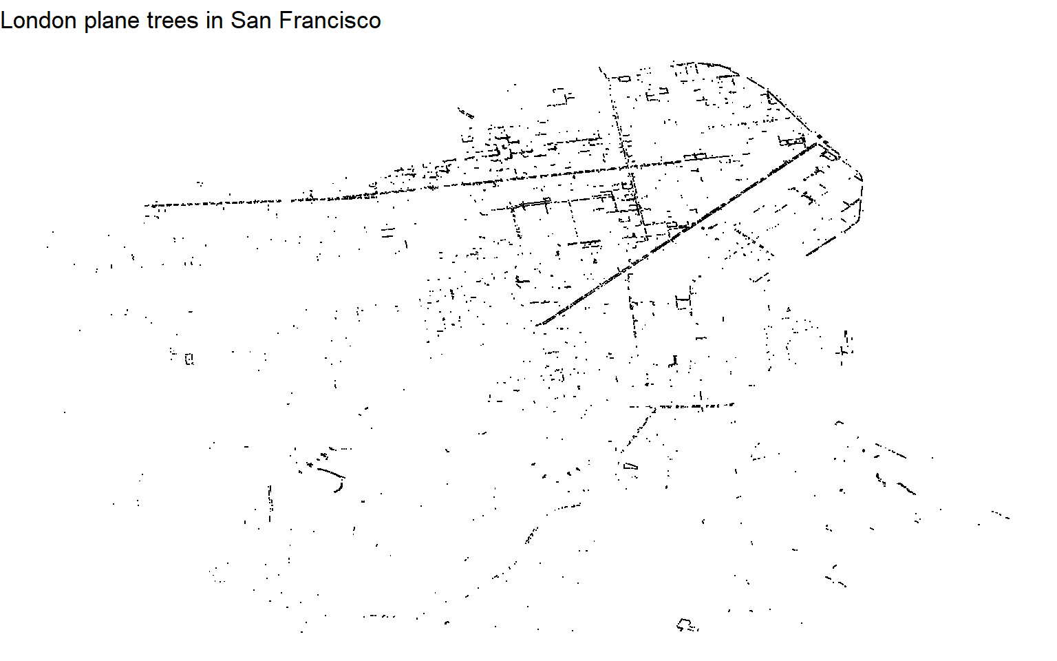

We get an okay sense of London planes from this map – it looks like they line streets or boulevards, especially in the city’s northeast. Having contextual clues, like land/water or roads, would make it easier to interpret. The downside of not having these clues becomes more obvious when looking at Ornamental Pear trees, which aren’t as common and tend not to line streets the same way London planes do.

sf_trees %>%
  filter(common_name == "Ornamental Pear") %>%
  ggplot(aes(longitude, latitude)) +
  geom_point(shape = ".") +
  labs(title = "Ornamental Pear trees in San Francisco") +
  theme_void()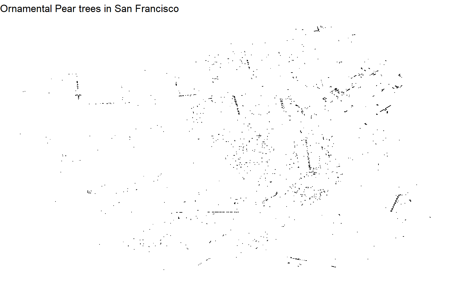

It’s almost useless, right? We need to know where the roads are.

Mapping roads

What is a shapefile?

We can add roads using a shapefile, which is format for geospatial data. I think of it as a way to store everything you might see on a road map – roads, rivers, lakes, cities, gas stations, parks, and other points of interest. It’s called a shapefile because it’s composed of different shapes, depending on what you’re trying to describe. Wikipedia’s shapefile page has an example that illustrates different shapes you might find in a shapefile:

Points to show wells
Lines to show rivers
Polygons to show the lake

shapefile example

Finding a shapefile for San Francisco roads

Usually a Google search of “<what you’re looking for> shapefile” will get you what you need. In our case, searching for “San Francisco roads shapefile” leads us to the US Census Bureau, which has exactly what we need: all roads in San Francisco county.

We need to download the zip file with all the files we need, then read the shapefile using the sf package’s read_sf() function. You can download and unzip the file manually if you like, but it’s possible to do it all in R, which is what we’ll do here. These are the steps:

Create a temporary directory and download the zipped file to it
Create a second temporary directory and unzip the file to that location
Use read_sf() to import the individual file we need

# 1. Create a temp directory and download ZIP file from US Census
temp_download <- tempfile()
download.file("https://www2.census.gov/geo/tiger/TIGER2017//ROADS/tl_2017_06075_roads.zip", temp_download)

# 2. Create a temp directory to unzip the file into
temp_unzip <- tempfile()
unzip(temp_download, exdir = temp_unzip)

# 3. Read the unzipped shapefile from the temporary filepath
sf_roads <- read_sf(paste0(file.path(temp_unzip), "/tl_2017_06075_roads.shp"))

Now that we have our roads shapefile, let’s see what it looks like. ggplot2 has a geom_sf() function for exactly these types of files. Unlike most other geometries, we don’t need to specify the aes() layer.

ggplot(sf_roads) +
  geom_sf()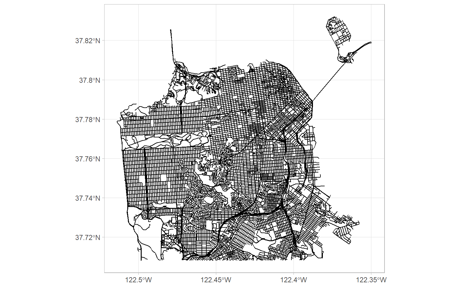

Looks great! This will add some useful context to our tree locations.

Combining tree locations and roads

Mapping all trees

To combine our our tree location data and roads shapefile, we need to feed them into the same ggplot() call. There are four things worth nothing in this code snippet:

The geom_sf() function needs to specify sf_roads as its source data
geom_point() is written after geom_sf(), which ensures that the points are plotted on top of the roads
We use coord_sf() to get the right aspect ratio
We use theme_void() as a “blank” theme, which is useful for maps

sf_trees %>%
  ggplot() +
  geom_sf(data = sf_roads, col = "grey90", alpha = 0.7) +
  geom_point(
    aes(longitude, latitude),
    shape = ".",
    alpha = 0.5,
    col = "darkgreen"
  ) +
  coord_sf() +
  labs(title = "Where are San Francisco's trees?") +
  theme_void()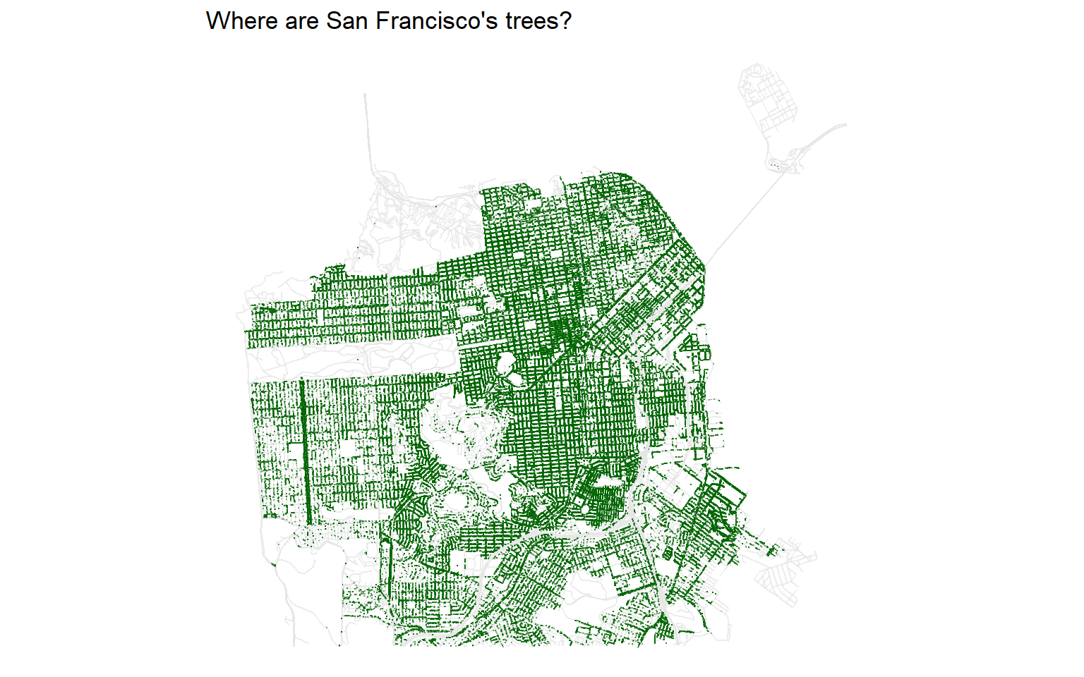

We can see some clear patterns, like a concentration of trees along a road in the western part of the city. This turns out to be Sunset Boulevard!

Mapping the nine most common tree species

I’m personally more curious about where different species of trees are, so let’s create small multiples of the nine most common tree species. We’ll do a few extra steps, like renaming one particularly long species name and adjusting the margins of some of the plot elements.

sf_trees %>%
  mutate(
    common_name = ifelse(
      common_name == "Indian Laurel Fig Tree 'Green Gem'",
      "Indian Laurel Fig",
      common_name
    ),
    common_name = fct_lump(common_name, 9)
  ) %>%
  filter(!is.na(common_name), common_name != "Other") %>%
  add_count(common_name, name = "tree_count") %>%
  mutate(common_name = fct_reorder(common_name,-tree_count)) %>%
  ggplot() +
  geom_sf(data = sf_roads, col = "grey90", alpha = 0.5) +
  geom_point(
    aes(longitude, latitude),
    shape = ".",
    alpha = 0.5,
    col = "darkgreen"
  ) +
  facet_wrap( ~ common_name) +
  coord_sf() +
  labs(title = "Where are San Francisco's trees?",
       subtitle = "Showing the nine most common tree species") +
  theme_void() +
  theme(
    plot.subtitle = element_text(margin = margin(b = 4, unit = "pt")),
    strip.text = element_text(size = 8, margin = margin(
      t = 2, b = 2, unit = "pt"
    ))
  )

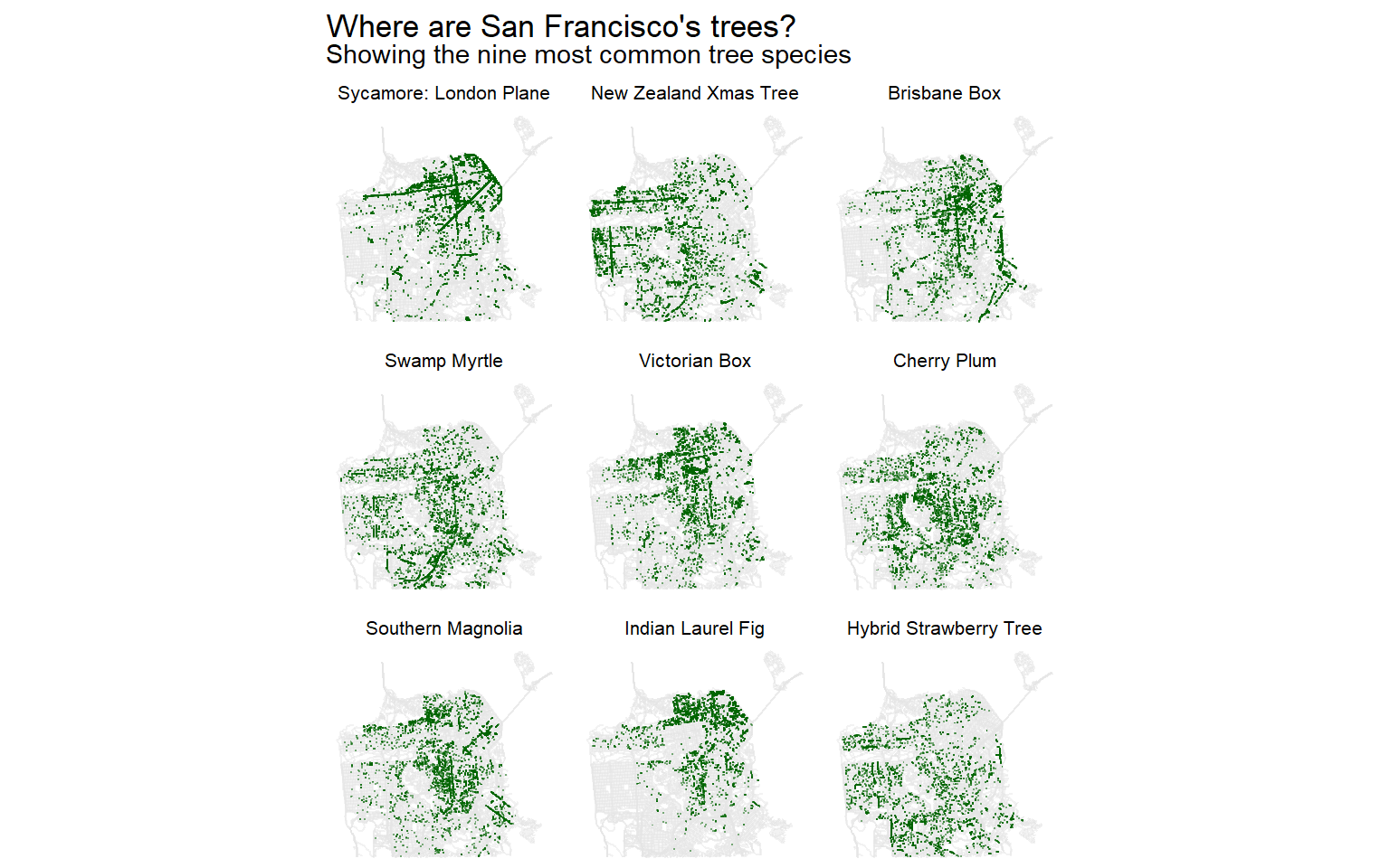
Personally, I think these small multiples of different species are more interesting and informative. For example, I wonder why London Plane and Indian Laurel Fig trees are so common in the northeast but relatively sparse in the south. That’s a question I wouldn’t know to ask if I were looking at the distribution of trees overall. I don’t know much about trees or San Francisco, so if you have any ideas, let me know on Twitter.

Conclusion

I hope you enjoyed what I tried to make a fairly gentle introduction to geographical mapping and shapefiles. If you liked this, check out the #TidyTuesday hashtag on Twitter or, even better participate yourself!