How dangerous is climbing Mount Everest?

Apr 6, 2020

data exploration / annotations / spineplots

In this series of posts, we will analyze climbing expeditions to the Himalayas, a mountain range comprising over 50 mountains, including Mount Everest, the tallest mountain in the world.

This is Part 2 of a two-part series:

Part 1 looked at Himalayan peaks and their first ascents
Part 2 (this post) looks at Everest expeditions

This post will focus on expeditions to Mount Everest, the most famous Himalayan peak and the tallest mountain in the world. Everest expeditions have received some mainstream media attention fairly recently, with reports about overcrowding and whether or not this overcrowding plays a role in the deaths of some climbers. (It’s an interesting topic – I recommend reading the linked articles.)

We will do our own exploration of Everest expeditions using data from The Himalayan Database. In particular, we’ll investigate:

How popular is Mount Everest?
What time of year do people climb?
How dangerous is climbing Everest?

Setup

First, we’ll load the tidyverse and some other useful packages:

fishualize for ggplot2 colour palettes inspired by fish
scales for turning ugly numbers into pretty numbers (e.g., 0.3 to 30%)
extrafont for additional fonts to use in graphs

We’ll also set a default ggplot2 theme and import our data.

library(tidyverse)
library(fishualize)
library(scales)
library(extrafont)
library(ggtext)

theme_set(theme_light())

peaks <- readr::read_csv("https://raw.githubusercontent.com/tacookson/data/master/himalayan-expeditions/peaks.csv")
expeditions <- readr::read_csv("https://raw.githubusercontent.com/tacookson/data/master/himalayan-expeditions/expeditions.csv")
members <- readr::read_csv("https://raw.githubusercontent.com/tacookson/data/master/himalayan-expeditions/members.csv")

Data inspection

We have two data tables to investigate: expeditions, which has data on entire climbing expeditions, and members, which has data on the individual members of those expeditions.

Let’s start with expeditions.

expeditions %>%
  glimpse()

## Rows: 10,364
## Columns: 16
## $ expedition_id      <chr> "ANN260101", "ANN269301", "ANN273101", "ANN27830...
## $ peak_id            <chr> "ANN2", "ANN2", "ANN2", "ANN2", "ANN2", "ANN2", ...
## $ peak_name          <chr> "Annapurna II", "Annapurna II", "Annapurna II", ...
## $ year               <dbl> 1960, 1969, 1973, 1978, 1979, 1980, 1980, 1981, ...
## $ season             <chr> "Spring", "Autumn", "Spring", "Autumn", "Autumn"...
## $ basecamp_date      <date> 1960-03-15, 1969-09-25, 1973-03-16, 1978-09-08,...
## $ highpoint_date     <date> 1960-05-17, 1969-10-22, 1973-05-06, 1978-10-02,...
## $ termination_date   <date> NA, 1969-10-26, NA, 1978-10-05, 1979-10-20, 198...
## $ termination_reason <chr> "Success (main peak)", "Success (main peak)", "S...
## $ highpoint_metres   <dbl> 7937, 7937, 7937, 7000, 7160, 7000, 7250, 6400, ...
## $ members            <dbl> 10, 10, 6, 2, 3, 6, 7, 19, 9, 5, 5, 5, 6, 4, 3, ...
## $ member_deaths      <dbl> 0, 0, 0, 0, 0, 1, 0, 0, 1, 0, 1, 0, 0, 0, 0, 0, ...
## $ hired_staff        <dbl> 9, 0, 8, 0, 0, 2, 2, 0, 3, 0, 0, 3, 4, 2, 0, 2, ...
## $ hired_staff_deaths <dbl> 0, 0, 0, 0, 0, 0, 0, 0, 0, 0, 0, 0, 0, 0, 0, 0, ...
## $ oxygen_used        <lgl> TRUE, FALSE, FALSE, FALSE, FALSE, FALSE, FALSE, ...
## $ trekking_agency    <chr> NA, NA, NA, NA, NA, NA, NA, NA, NA, NA, NA, "Kun...

expeditions has four types of data:

Basic data on the peak. We could bring in the peaks table if we wanted information like alternative names or heights.
Important expedition dates – when they reached basecamp, when they reached the summit, and when the expedition ended
“Outcomes”, including elevation highpoint and the reason for the expedition ending
Miscellaneous additional data, like number of members, deaths, and whether oxygen was used

What about expedition members?

members %>%
  glimpse()

## Rows: 76,519
## Columns: 21
## $ expedition_id        <chr> "AMAD78301", "AMAD78301", "AMAD78301", "AMAD78...
## $ member_id            <chr> "AMAD78301-01", "AMAD78301-02", "AMAD78301-03"...
## $ peak_id              <chr> "AMAD", "AMAD", "AMAD", "AMAD", "AMAD", "AMAD"...
## $ peak_name            <chr> "Ama Dablam", "Ama Dablam", "Ama Dablam", "Ama...
## $ year                 <dbl> 1978, 1978, 1978, 1978, 1978, 1978, 1978, 1978...
## $ season               <chr> "Autumn", "Autumn", "Autumn", "Autumn", "Autum...
## $ sex                  <chr> "M", "M", "M", "M", "M", "M", "M", "M", "M", "...
## $ age                  <dbl> 40, 41, 27, 40, 34, 25, 41, 29, 35, 37, 23, 44...
## $ citizenship          <chr> "France", "France", "France", "France", "Franc...
## $ expedition_role      <chr> "Leader", "Deputy Leader", "Climber", "Exp Doc...
## $ hired                <lgl> FALSE, FALSE, FALSE, FALSE, FALSE, FALSE, FALS...
## $ highpoint_metres     <dbl> NA, 6000, NA, 6000, NA, 6000, 6000, 6000, NA, ...
## $ success              <lgl> FALSE, FALSE, FALSE, FALSE, FALSE, FALSE, FALS...
## $ solo                 <lgl> FALSE, FALSE, FALSE, FALSE, FALSE, FALSE, FALS...
## $ oxygen_used          <lgl> FALSE, FALSE, FALSE, FALSE, FALSE, FALSE, FALS...
## $ died                 <lgl> FALSE, FALSE, FALSE, FALSE, FALSE, FALSE, FALS...
## $ death_cause          <chr> NA, NA, NA, NA, NA, NA, NA, NA, NA, NA, NA, NA...
## $ death_height_metres  <dbl> NA, NA, NA, NA, NA, NA, NA, NA, NA, NA, NA, NA...
## $ injured              <lgl> FALSE, FALSE, FALSE, FALSE, FALSE, FALSE, FALS...
## $ injury_type          <chr> NA, NA, NA, NA, NA, NA, NA, NA, NA, NA, NA, NA...
## $ injury_height_metres <dbl> NA, NA, NA, NA, NA, NA, NA, NA, NA, NA, NA, NA...

members also has four types of data:

Some of the same data from the peaks and expeditions tables, here for convenience
Demographic data, like age and sex
Individual outcomes, like elevation high and unfortunate “outcomes” like injury and death
Miscellaneous additional data, like expedition role and whether the individual used oxygen

Now that we have a general sense of our data, let’s create “Everest versions” of expeditions and members. Then, we can start answering our questions.

everest_expeditions <- expeditions %>%
  filter(peak_name == "Everest")

everest_members <- members %>%
  filter(peak_name == "Everest")

How popular is Mount Everest?

As I noted in the introduction, media outlets like the BBC and the New York Times have reported on criticisms of overcrowding at Mount Everest. Just how crowded is it? And how has that changed over time? Let’s look at the number of expeditions and the number of climbers each year since the first recorded expedition in 1921.

everest_expeditions %>%
  group_by(year) %>%
  # Capitalizing names so they'll look nice in the graph
  summarise(Expeditions = n(),
            Climbers = sum(members + hired_staff)) %>%
  ungroup() %>%
  # There are implicit zeros, especially before 1950
  # Use complete() to turn them into explicit zeros
  complete(year = 1920:2019,
           fill = list(Expeditions = 0, Climbers = 0)) %>%
  gather("category", "number", -year) %>%
  ggplot(aes(year, number, fill = year)) +
  geom_col() +
  facet_wrap( ~ category, scales = "free_y") +
  scale_x_continuous(breaks = seq(1920, 2020, 10)) +
  scale_y_continuous(labels = label_comma()) +
  scale_fill_fish(option = "Pseudocheilinus_tetrataenia",
                  direction = 1) +
  labs(
    title = "Everest's popularity has soared since the 1980s",
    caption = "Source: The Himalayan Database",
    x = "",
    y = ""
  ) +
  theme(
    legend.position = "none",
    text = element_text(family = "Bahnschrift"),
    panel.grid.minor = element_blank(),
    strip.text = element_text(size = 12, colour = "black"),
    strip.background = element_blank()
  )

## `summarise()` ungrouping output (override with `.groups` argument)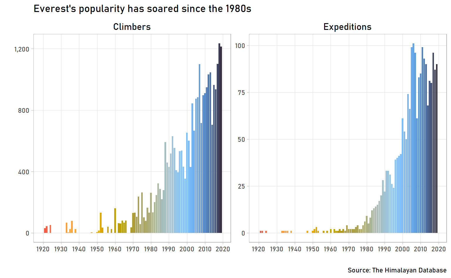

The graphs themselves look like mountains! Everest has become much more popular since the 1980s. For the past 20 years, a typical year would see about 75-100 expeditions comprising 800-1,200 climbers.

What time of year do people climb?

Many parts of the world are nicer to visit during certain times of the year. If you visit Toronto, Canada (my hometown), a July trip will be a much different experience than a November trip. Is Mount Everest any different?

everest_expeditions %>%
  mutate(
    decade = year %/% 10 * 10,
    season = fct_relevel(season, "Spring", "Summer", "Autumn", "Winter")
  ) %>%
  count(decade, season, name = "expeditions") %>%
  ggplot(aes(decade, expeditions, fill = season)) +
  geom_col() +
  scale_x_continuous(breaks = seq(1920, 2010, 10)) +
  scale_fill_fish(option = "Pseudocheilinus_tetrataenia",
                  discrete = TRUE,
                  direction = -1) +
  facet_wrap(~ season) +
  labs(
    title = "Spring is the most popular time to climb Mount Everest",
    subtitle = "Number of expeditions (1921-2019)",
    caption = "Source: The Himalayan Database",
    x = "",
    y = ""
  ) +
  theme(
    legend.position = "none",
    text = element_text(family = "Bahnschrift"),
    panel.grid.minor = element_blank(),
    strip.text = element_text(size = 12, colour = "black"),
    strip.background = element_blank()
  )

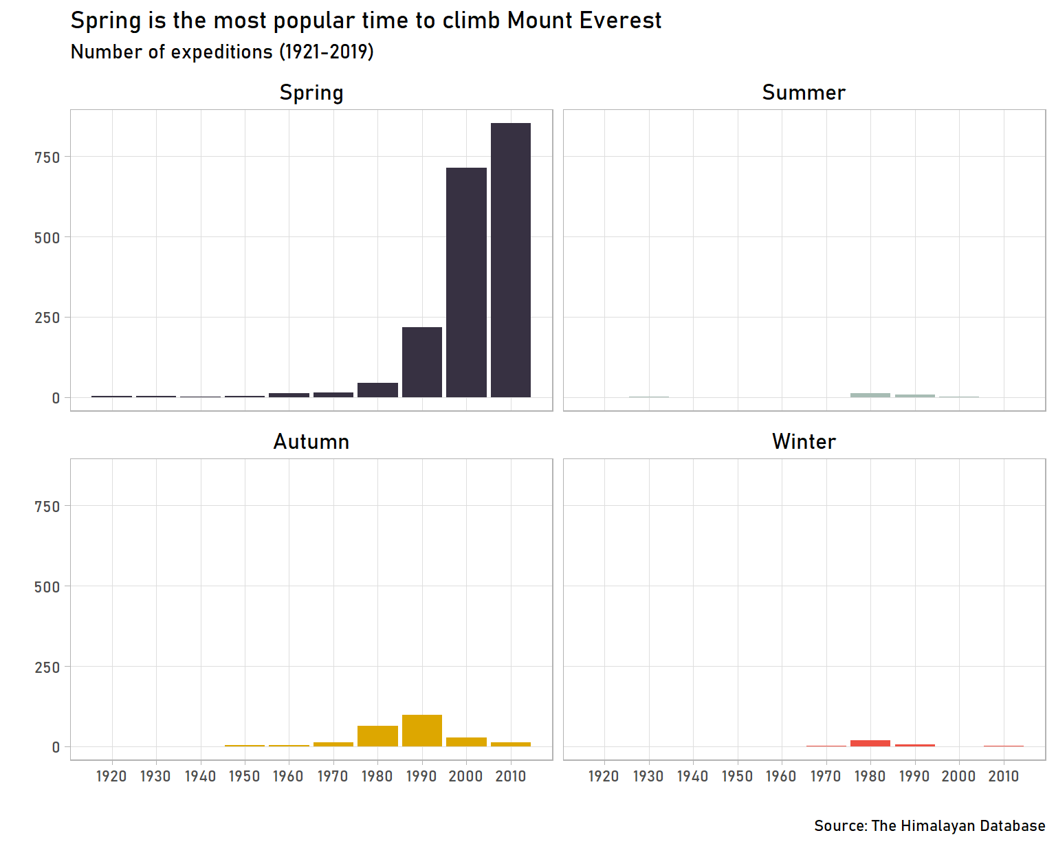
Spring expeditions are by far the most common. There are almost no expeditions during the summer, likely because it is monsoon season, a period with obviously less-than-ideal conditions for an arduous, weather-dependent climb. In fact, according to an article in Popular Mechanics, May is generally considered the best month to climb because it has the best weather – lower wind speeds and higher temperatures. Our data supports this idea: looking at expeditions we have a highpoint date for, almost 80% of them are in May.

everest_expeditions %>%
  filter(!is.na(highpoint_date)) %>%
  mutate(highpoint_month = lubridate::month(highpoint_date, label = TRUE)) %>%
  ggplot(aes(highpoint_month, y = ..prop.., group = 1)) +
  geom_bar(stat = "count",
           fill = "#373142FF", alpha = 0.7) +
  scale_y_continuous(breaks = seq(0, 0.8, 0.1),
                     labels = label_percent(accuracy = 1)) +
  labs(
    title = "Almost 80% of Everest expeditions were in May",
    subtitle = "Percent of expeditions by month of reaching their highpoint (1921-2019)",
    caption = "Source: The Himalayan Database",
    x = "",
    y = ""
  ) +
  theme(text = element_text(family = "Bahnschrift"),
        panel.grid.minor = element_blank())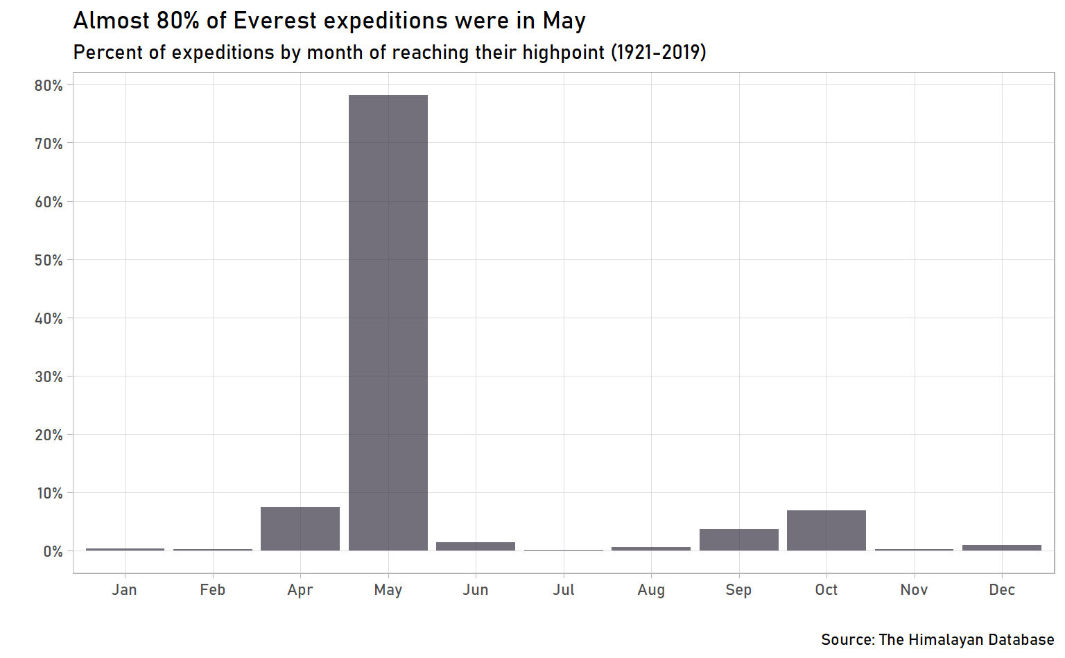

However, autumn climbing was more popular in the late 20th century. In fact, in the 1980s, the majority of expeditions took place during autumn.

everest_expeditions %>%
  filter(year >= 1960) %>%
  mutate(
    decade = paste0(year %/% 10 * 10, "s"),
    season = fct_relevel(season, "Spring", "Summer", "Autumn", "Winter")
  ) %>%
  count(decade, season, name = "expeditions") %>%
  group_by(decade) %>%
  mutate(pct_expeditions = expeditions / sum(expeditions)) %>%
  ungroup() %>%
  ggplot(aes(season, pct_expeditions, fill = season)) +
  geom_col() +
  scale_y_continuous(breaks = seq(0, 1, 0.2),
                     labels = label_percent(accuracy = 1)) +
  scale_fill_fish(option = "Pseudocheilinus_tetrataenia",
                  discrete = TRUE,
                  direction = -1) +
  facet_wrap(~ decade) +
  labs(
    title = "Autumn expeditions were more popular in the '70s, '80s, and '90s",
    subtitle = "Percent of expeditions by season (1921-2019)",
    caption = "Source: The Himalayan Database",
    x = "",
    y = ""
  ) +
  theme(
    legend.position = "none",
    text = element_text(family = "Bahnschrift"),
    panel.grid.minor = element_blank(),
    strip.text = element_text(size = 12, colour = "black"),
    strip.background = element_blank()
  )

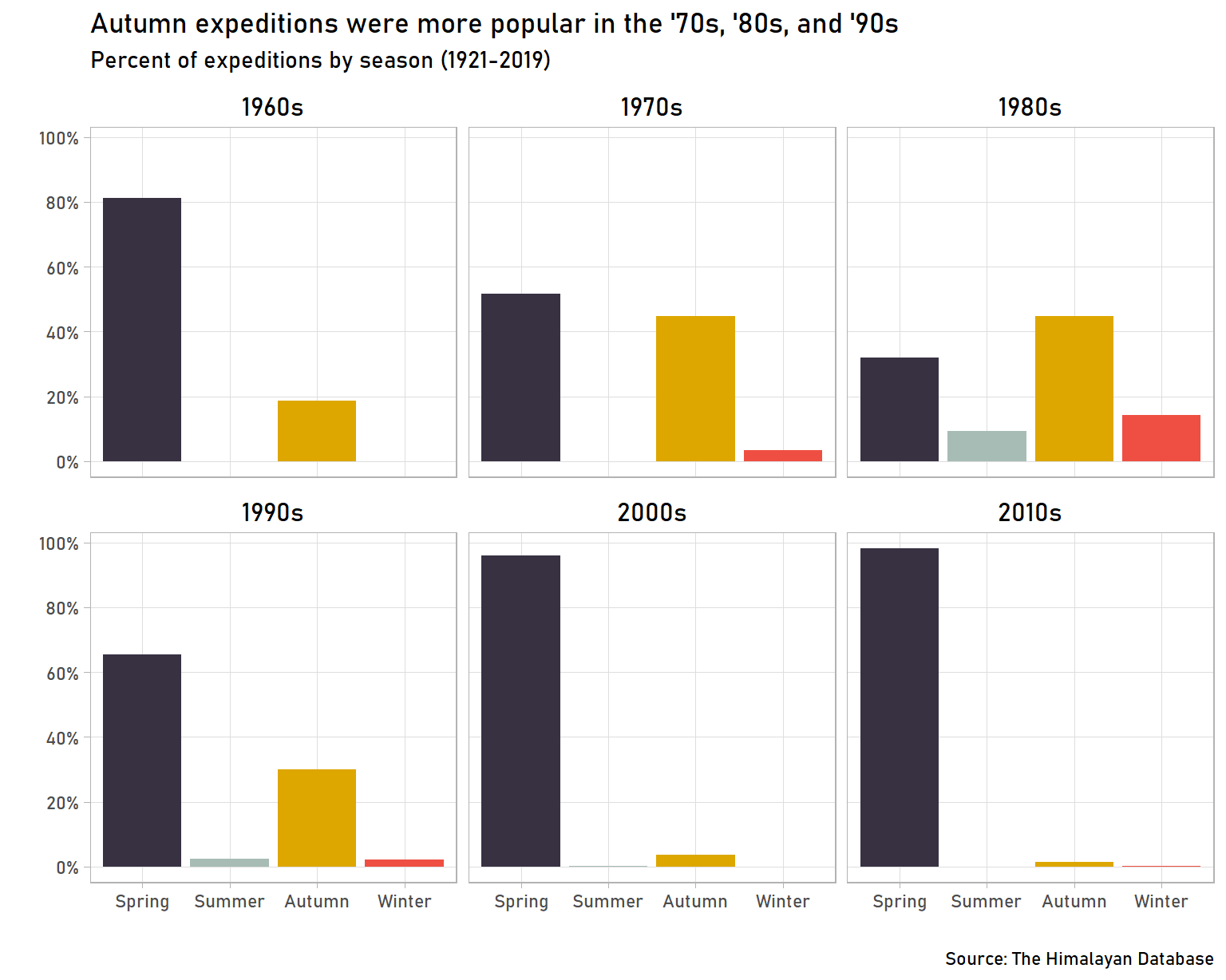
Why? I don’t know, but I have a guess. A 2003 article in The American Alpine Journal notes that 1963-1990s was “an era of bold climbing”, with many climbers attempting alternative routes. Maybe these alternatives routes were more feasible in the autumn or bold climbers sought out the novelty and challenge of an autumn climb.

How dangerous is climbing Everest?

People die climbing Mount Everest. It is physically arduous and the conditions are extremely harsh. The most recent climbing season – 2019 as of the time of this writing – saw 11 deaths. Many mainstream media outlets wrote stories on the topic, including this one from The Associated Press. How does the 2019 season compare to others?

everest_members %>%
  count(year, wt = died, name = "died") %>%
  complete(year = 1921:2019, fill = list(died = 0)) %>%
  ggplot(aes(year, died)) +
  geom_line(size = 0.8, col = "#FF9A41") +
  geom_point(size = 2, col = "#FF9A41") +
  geom_label(
    aes(1931, 7),
    label = "1922 avalanche",
    fill = "white",
    label.size = NA,
    family = "Bahnschrift"
  ) +
  geom_label(
    aes(1988, 15),
    label = "1996 blizzard",
    fill = "white",
    label.size = NA,
    family = "Bahnschrift"
  ) +
  geom_label(
    aes(2005, 17),
    label = "2014 avalanche",
    fill = "white",
    label.size = NA,
    family = "Bahnschrift"
  ) +
  scale_x_continuous(breaks = seq(1920, 2020, 10)) +
  labs(
    title = "For decades, at least one person has died climbing Everest",
    subtitle = "Number of deaths from Everest expeditions (1921-2019)",
    caption = "Source: The Himalayan Database",
    x = "",
    y = ""
  ) +
  theme(
    text = element_text("Bahnschrift"),
    panel.grid.minor.y = element_blank(),
    axis.text = element_text(size = 12)
  )

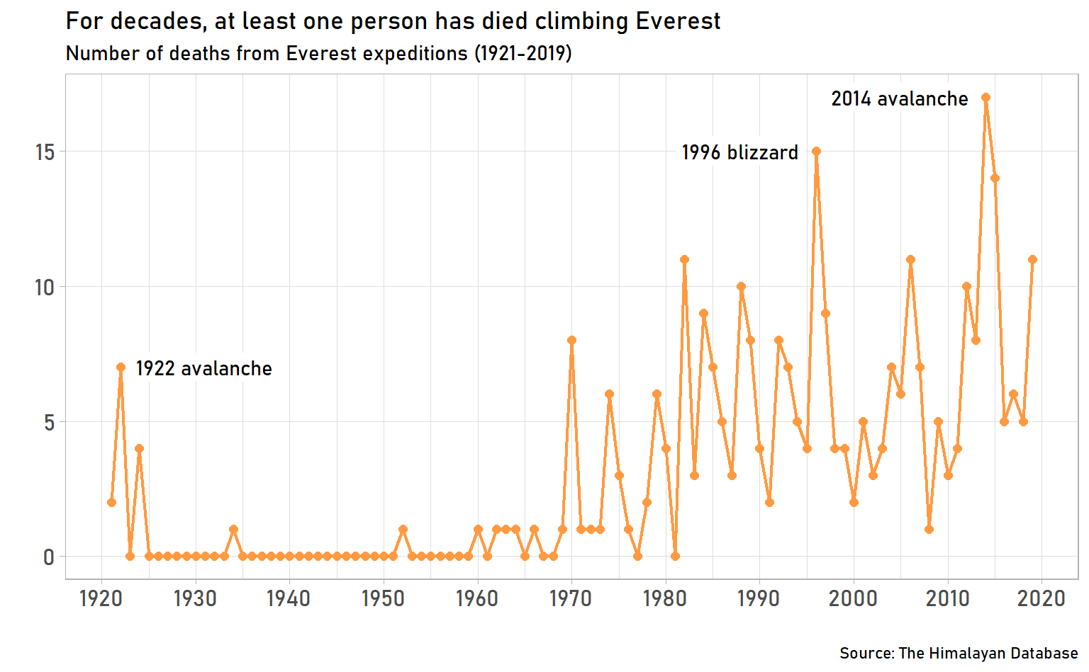
It looks like 11 deaths in a season is a high, but not extraordinary, figure. Two seasons in the previous 5 years had more deaths. This includes 2014, the year with 17 deaths – the most ever in a single year – 16 of which were the result of a single avalanche. Previous seasons with high death counts include 1996, when a group of climbers was caught in a blizzard, and 1922, when an avalanche killed 7 members of the British expedition attempting the summit.

These single-event catastrophes raise another question: What are the main causes of death? We have the data to answer that question, though we will limit our scope to make sure we have an effective visualization. First, we’ll look only at expeditions since the 1970s, since that is when we started seeing consistent expeditions every year.

Second, we’ll look at the top five causes of death and lump the rest into a category called “Other”. We do this to keep the visualization from looking messy and therefore difficult to read.

Third, we’ll look at deaths by decade instead of by year. Looking at annual figures is quite noisy, making it difficult to see the overall trend. (Though if you’re curious, I encourage you to re-create the visualization using annual figures – see what it looks like.

everest_members %>%
  filter(died, year >= 1970) %>%
  mutate(death_cause = fct_lump(death_cause, 5)) %>%
  count(decade = year %/% 10 * 10, death_cause) %>%
  complete(decade, death_cause, fill = list(n = 0)) %>%
  group_by(decade) %>%
  mutate(pct = n / sum(n)) %>%
  ungroup() %>%
  mutate(death_cause = fct_reorder(death_cause, n, sum)) %>%
  ggplot(aes(decade, pct, fill = death_cause)) +
  geom_area() +
  scale_x_continuous(labels = label_number(big.mark = "", suffix = "s")) +
  scale_y_continuous(labels = label_percent()) +
  scale_fill_fish(option = "Pseudocheilinus_tetrataenia", discrete = TRUE) +
  labs(
    title = "Avalanches and falls can be particularly deadly",
    subtitle = "Percent of deaths by cause of death (1960-2019)",
    caption = "Source: The Himalayan Database",
    x = "",
    y = "",
    fill = "Cause of death"
  ) +
  theme_minimal() +
  theme(text = element_text(family = "Bahnschrift"),
        axis.text = element_text(size = 12),
        panel.grid.minor = element_blank())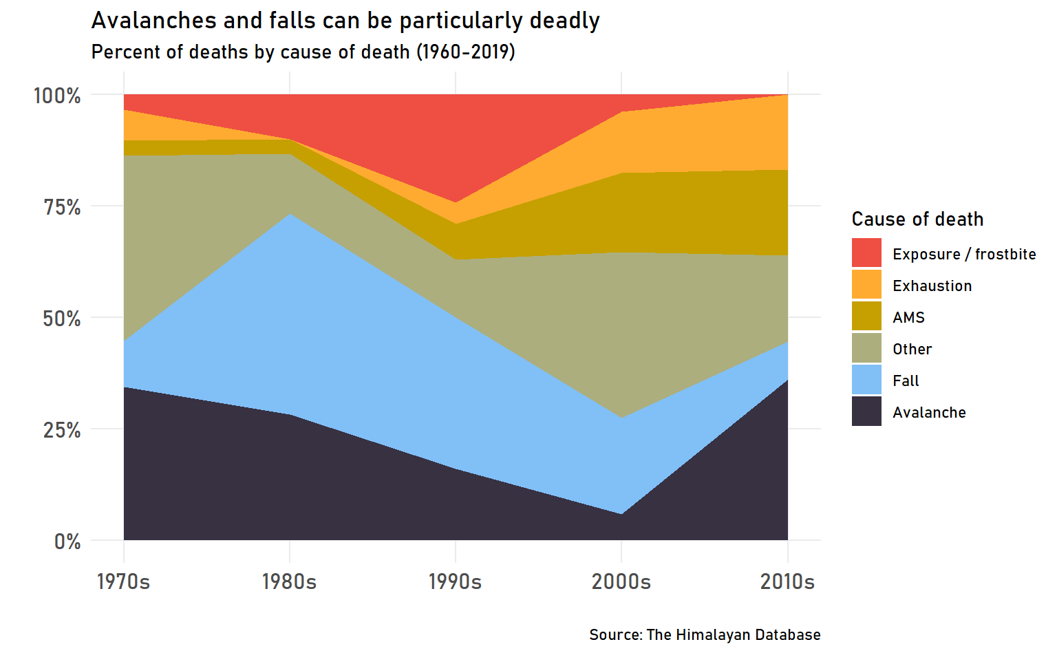

Overall, it looks like weather and conditions are the main thing to be worried about, with falls and avalanches being particularly deadly. (I’m guessing that falls are associated with windy or otherwise poor conditions, though perhaps they could also be associated with less experienced climbers.) In the 1980s, falls and avalanches were responsible for 3 in 4 deaths and in other decades they account for around half of deaths. It also looks like exhaustion and AMS – Acute Mountain Sickness – have become more prevalent in the last 20 years. Maybe this is a consequence of less experienced climbers attempting Everest and getting into situations they aren’t prepared for. If you are climbing Everest, there is a lot to wary of.

Conclusion

We’ve learned some things about Everest expeditions, including their rise in popularity, the trends in when climbers attempt embark on their expeditions, and some details on the dangers associated with climbing. We could look at so many more aspects, including:

What is the composition of expeditions? For example, how big do they tend to be and what proportion consist of hired staff?
What injuries are associated with climbing Everest?
Are there characteristics of climbers associated with higher or lower death rates? For example, are Sherpas – presumably well-acclimated to high altitudes – less likely to suffer from AMS?
What are the general trends in solo expeditions and the use of oxygen?

If you’re curious about these (or other questions!), please use this data to look into them yourself and let me know on Twitter. And, if you enjoyed this post, I encourage you to read the other post analyzing this dataset, which looks at Himalayan peaks and their first ascents.